Abstract
This document presents a concise, efficient and intuitive process for establishing LiDAR project data requirements, incorporating them into a request for proposal (RFP) and assessing the data against those requirements. An overview of LiDAR technology and data uncertainty provides insight into the reasoning behind point cloud and calibrated image data requirements. Suggested text for applying these requirements within the context of a request for proposal (RFP) is given. Methods for assessing the spatial orientation of the data yield a well-documented lineage from the data to network survey control coordinates. Additional methods are presented to assess the fundamental characteristics of point clouds and calibrated images assuring extracted features, measurements and models will meet project requirements. Examples employing TopoDOT® software tools demonstrate the execution of each process. The examples contained herein are predominately for civil infrastructure applications although the methods may be broadly applied in other areas.
Contents
- Introduction
- LiDAR Data Uncertainty
- Establishing LiDAR System Data Requirements
- LiDAR System Data Characteristics
- Summary
Introduction
LiDAR scanning systems are quickly emerging as a mainstream technology in civil infrastructure applications. Data is typically acquired as a point cloud and is often accompanied by calibrated images.
The fundamental difference between a “survey coordinate” and “point cloud coordinate”, is that the survey coordinate has attribute intelligence and the point cloud coordinate does not. That is to say a professional surveyor identified the survey feature, aimed an instrument at that point, acquired its location and documented it.
Point clouds are made up of samples acquired within a scene with no intelligence on any single point. This has made the evaluation of LiDAR data against some established control survey data problematic. Thus there is significant interest among LiDAR data “Customers” in establishing data requirements, articulating requirements within a Request for Proposal (RFP) and extracting quantifiable metrics from the data for assessment against those requirements to assure features, measurements and models extracted from the LiDAR data will meet overall infrastructure project objectives.
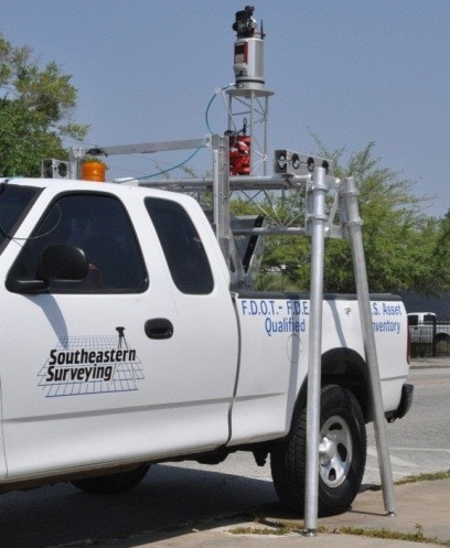
Terrestrial Mobile LiDAR System: Courtesy R.E.Y. Engineers CA
Within complex LiDAR systems, field operations and processing workflows exist numerous potential sources of data uncertainty. Without clear requirements on LiDAR data and methods for extracting metrics from the data, Customers typically shift their focus and requirements to the CAD deliverable extracted from the data. This reliance on the CAD model often decreases productivity and performance across the entire process.
In this process any inaccuracies resulting from survey blunders, modeling mistakes, or other anomalies are identified in the CAD model and thus are not found until after the time and expense has been applied to the extraction operation. Deliverable extraction is relatively labor intensive and time-consuming. Should the CAD deliverable fail to meet requirements, the source of the error is often unclear as it could be the LiDAR data, an error in the modeling process or both. This can lead to confusion, delayed schedules and even a general mistrust in LiDAR technology itself.
Feeding downstream operations with the CAD model alone tends to require expensive “over-modeling” of the data. Customers without the capability to extract basic measurements, features or models tend to request the extraction of significantly more complex and extensive CAD models. This reliance on the CAD deliverable is understandable in that it feeds the downstream design processes and fits directly into standard design workflows. Thus it’s not uncommon for a Customer to avoid the LiDAR data altogether depending entirely on the delivered CAD model. Despite the model meeting acceptance criteria, the Customer’s avoidance of the point cloud data typically results in additional processing time and expense.
In contrast, a processing program such as TopoDOT® allows the Customer to extract features and measurements directly from the LiDAR data. These features are extracted where, when and in the form required to directly meet the needs of the downstream design and engineering processes. For example, should additional extensive modeling be required in certain areas, designers and engineers with access to the LiDAR data can communicate specific requirements for the extracted models to the CAD processing technician. Thus the ultimate effect of the Customer directly using LiDAR data in downstream operations replaces over-modeling with a more optimized, efficient and less costly modeling process.
Given the benefits associated with direct evaluation of LiDAR data and employing that data in downstream processes, the Customer clearly requires the capability to express LiDAR data requirements within a proposal and evaluate the acquired data against those requirements. Certainty 3D’s experience in supporting hundreds of successful LiDAR projects has yielded a very concise, efficient and intuitive process for achieving these objectives. Tools implemented in Certainty 3D’s TopoDOT® software support the effective implementation of this process for static, terrestrial mobile and airborne LiDAR system platforms.
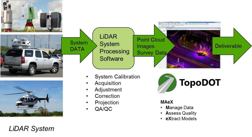
Illustrated above is the fundamental data flow from the LiDAR system into TopoDOT® processing software. This document focuses primarily on the “ASSESS” component of the Certainty 3D “MAeX” workflow. This Assess process offers the Customer “pass/fail” acceptance criteria for the LiDAR data. Should data fail to meet the Customer’s requirements it should be returned to the Consultant for adjustment at the system level.
This approach is consistent with LiDAR data’s status as “survey” data and as such should not be modified outside the oversight of the responsible Consultant. As a practical matter, the LiDAR system and process complexity combined with the tight accuracy requirements typically preclude TopoDOT® or any other third party software from modifying the data effectively since the source of data uncertainty is not reliably observable from the data alone.
LiDAR Data Uncertainty
This section provides an overview of LiDAR technology and sources of LiDAR data uncertainty. Understanding the potential for numerous sources of uncertainty will support the preceding claim that identifying its source(s) is impractical through access to the data alone. Furthermore, this information will provide a solid foundation for understanding subsequent discussions regarding the establishment of LiDAR data requirements.
Basic LiDAR Scanner Function
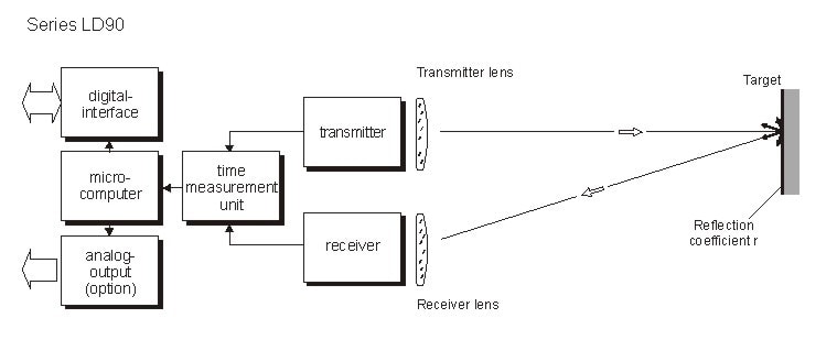
Laser rangefinder technology is the heart of a LiDAR scanner. For longer distance civil applications the rangefinder employs pulse time-of-flight technology. Basically a very short duration large amplitude pulse is emitted from the laser transmitter. The pulse is reflected from an arbitrary surface with a small portion of that energy returning to the receiver. Knowing the speed of light gives the distance between the rangefinder and reflecting surface.
A LiDAR scanner is implemented by directing the laser beam in a known direction within the scanner’s own coordinate system. In this way individual measurements are essentially vectors of known length. The resulting endpoint vector coordinates collectively comprise the point cloud.
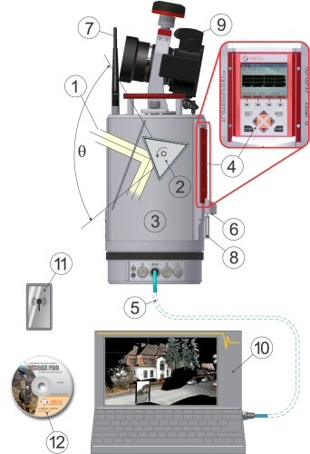
As an example, see the image of the Riegl VZ400 system. A triangular spinning mirror directs the rangefinder laser beam vertically over approximately 100 degrees per surface. Thus one complete mirror rotation results in three separate lines of point cloud data each over a hundred degree angle. This “fishtail” type scan pattern is then rotated in the orthogonal direction as the entire unit (#3) rotates 360 degrees about the base. Thus the rangefinder beam is accurately directed in a 100 x 360 degree scan pattern. In the case of the Riegl VZ400 these individual rangefinder measurements are acquired at about 300,000 points per second.
Note that other LiDAR scanners will offer slightly different mirror and scanning configurations. But the fundamental configuration of a single spinning mirror rotating orthogonally about a base is very common.
Origins of Data Uncertainty
In order to establish meaningful LiDAR data project requirements, one should understand the nature of data “uncertainty”. Our primary objective is that these concepts are easily understood and applied within the practical application of LiDAR technology to civil infrastructure or similar projects. Thus very rigorous analytics “not” adding to the practical application of LiDAR technology have been avoided.
We begin by defining the uncertainty of a specific point within a “point cloud” as being comprised of components; specifically a random and systematic component. So the uncertainty, µ, of any point is given by:
µtotal = µrandom + µsystematic
Thus µtotal is some expected distance between the acquired data point and the point’s actual location in the scene.
One should think of random error as being caused by anything resulting in the oscillation of the data about a relatively consistent mean value. For example, such oscillations could be caused by laser rangefinder noise and/or uncompensated vibration of the sensor platform. Random error oscillates between successive points within the point cloud. The characteristics of the oscillation are Gaussian in nature (bell curve). Within the practical application of LiDAR data, this oscillation is often described as “fuzziness” as the data exhibits a thickness far exceeding the roughness of a flat wall, road, sidewalk, or similar surface.
Rangefinder Uncertainty
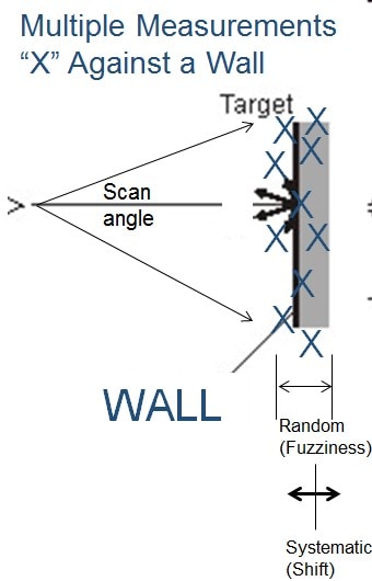
The illustration shown here is a simple diagram of the rangefinder laser beam being scanned vertically along a flat wall. Each measurement is represented by an “X”. Long or short measurements thus represent the wall with some thickness (fuzziness).
Systematic rangefinder error can be thought of as an “offset” in the data. This error is typically caused by internal sensor component drift or incorrect calibration. Systematic error is typically low frequency or even constant in nature. Thus points in close proximity are all affected in the same direction and magnitude resulting in “shifts” in the data from the true location. In this simple example, any position deviation between a line fit to the “X” data and the actual wall location would be considered a systematic error.
Static LiDAR Uncertainty
Additional sources of random and systematic error are associated with the field process for acquiring static LiDAR data. Random errors might be caused by oscillating movement of the platform whether it is a tripod, TopoLIFT™ or other stationary platform. For example a tripod might sit atop a bridge which vibrates with passing traffic. High winds can also result in platform movement. Such movement will manifest itself in some type of corresponding oscillation in the LiDAR data. These are just two examples of potential sources of random uncertainty in the acquired LiDAR data.
Systematic uncertainty introduced by static platform operation will typically result from field process anomalies such as improper reference target setup, slow non-oscillating movement of the platform (sinking), and survey errors. Typically LiDAR scanners locate reference targets tied to survey control coordinates to determine their orientation within the project coordinate system. Thus any reference control survey errors resulting from ineffective network design, data adjustment process or blunders might propagate to systematic errors in the acquired LiDAR data.
Terrestrial Mobile LiDAR Uncertainty
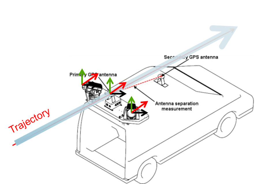
Mobile LiDAR systems are considerably more complex than static systems. Global Positioning System (GPS) receivers, an inertial measurement unit (IMU) and other sensors determine a moving vehicle’s position and orientation along a path with no external references other than GPS. This path is typically referred to as the “trajectory”. LiDAR scanners and cameras are mounted to the platform in order to acquire the point cloud and images as the vehicle moves along its trajectory.
The system illustration below indicates the many sensor coordinate systems which must be known and calibrated accurately to the primary platform coordinate system. In this illustration there are two LiDAR scanners, an IMU and GPS. Calibration of each system requires that the relative position and orientation of each component within the platform coordinate system must be known very accurately; typically to within a few hundredths of a degree.
There are numerous potential sources of systematic uncertainty within a mobile LiDAR system. Fixed data offsets can be caused by relative misalignment of the platform sensors. A loss of GPS signal can cause significant trajectory errors resulting in fixed non-constant but low frequency data offsets. One should keep in mind that these uncertainties require dramatically more processing to correct than those of static LiDAR platforms. These adjustments are typically non-linear and require very sophisticated processing algorithms tied closely to the system.
Random noise might be introduced into this mobile LiDAR system in several ways. A primary source may be the rangefinder noise associated with each laser scanner. Another example might be flexing of the system platform whereby the relative sensor orientation in the platform coordinate frame is oscillating in an unknown way. Another cause might be an IMU of insufficient bandwidth to compensate accurately for vehicle motion. Random uncertainty or “fuzziness” in the LiDAR data could be caused by any one or combination of these or similar system performance anomalies.
This brief overview of LiDAR data uncertainty is intended to provide a basic understanding of the discussion to follow regarding the establishment of LiDAR system data requirements. One should also appreciate the overall complexity of these systems, the numerous potential sources of data uncertainty and that the source(s) of data uncertainty is typically not identifiable from the data alone. Thus any expectation of compensating for these uncertainties using only the LiDAR data is generally not feasible. This is especially true when requirements for infrastructure design and construction applications demand very high accuracy. As mentioned previously, such adjustments should be made at the system level by the responsible Consultant.
Establishing LiDAR System Data Requirements
The Customer should establish data requirements consistent with meeting their overall project objectives. These requirements should be clearly defined along with the intended process for their respective evaluation. Typically these requirements are communicated to the Consultant within the content of a request for proposal (RFP).
A LiDAR data set is generally comprised of three components: 1) point cloud data, 2) survey control data and 3) calibrated images (if available). Certainty 3D’s experience consistently shows there are only six characteristics necessary to assess whether the LiDAR data meets the project requirements. These characteristics are easily extracted, quantified, and interpreted. They are:
- Scan (static) or Flightline (mobile) alignment
- Survey control alignment
- Calibrated image alignment
- Random noise
- Point density
- Coverage
The first three characteristics: Scan/Flightline alignment, Survey control alignment and image alignment collectively establish a traceable lineage between the images, point cloud and survey control coordinates. The latter three: Random noise, Point density and Coverage refer to LiDAR data characteristics necessary to assure extracted features, measurements and/or models will be of sufficient fidelity to meet project requirements.
Establishing Lineage to Survey Control
In this section the method for establishing a traceable lineage yielding quantifiable metrics between the point cloud and survey control coordinates is described for both static and mobile LiDAR data. These data sets have inherently different structures and therefore require different approaches in establishing the lineage between data and control.
This lineage is critical as the control survey is typically the only “sealed” document attesting to the accuracy of the entire LiDAR project. TopoDOT® offers “Control to Point Cloud Analysis” and “Flightline Assessment” tools along with techniques specifically designed to establish this lineage in a straightforward and intuitive way.
Static LiDAR Data
TopoDOT® offers tools and a relatively simple two-step process to establish lineage between a static LiDAR data point cloud and survey control coordinates. Moreover these processes yield quantifiable and easily understood metrics.
Step 1: Static LiDAR Data to Survey Control Alignment
As mentioned in previous sections, static LiDAR scanners determine their position and orientation by locating reference targets tied to survey control coordinates. These measurements may be supplemented with on-board sensors measuring level or compensators maintaining level. The data acquired from each scan position can be thought of as a “rigid” body requiring only linear displacements and rotations to achieve proper orientation within the project coordinate system.
Typically any direct comparison between a control coordinate and a specific point in the point cloud is problematic. While a surveyor identifies and selects each control coordinate, LiDAR systems do not intelligently select their measurements. Thus the probability of any single point cloud coordinate acquired at the same location as the control coordinate is extremely low. Therefore some form of modeling of the point cloud is necessary to extract a meaningful comparison between the control coordinate and point cloud data.
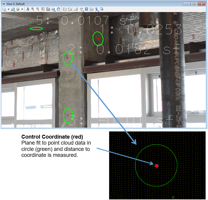
A very intuitive method begins by assuring that control coordinates are located such that the surrounding surface within close proximity is reasonably flat. This might be a wall, a floor, a ceiling, a sidewalk or a building. Then all data points within a sphere centered at the control coordinate can be best fit with a plane. The distance between the control coordinate and the plane can then be easily calculated. This analysis at an individual point measures distance in a single direction orthogonal to the plane. Supplementing this analysis with additional control coordinates located at planes oriented in other directions will ultimately provide an excellent assessment of the “rigid” point cloud orientation.
TopoDOT® offers the “point cloud to data analysis” tool which automatically executes this process at each control coordinate location. A summary report documents the distance from each coordinate to the nearest plane along with the average distance and standard deviation.
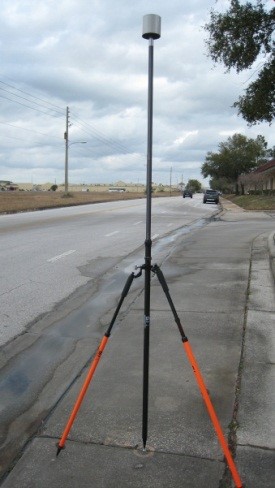
In roadway topography and similar applications, it can be problematic and time consuming to survey control coordinates on vertical services. For that reason coordinates are typically marked along the roadway or nearby sidewalk surface. Reference targets atop rods are set up vertically over the coordinate location. In this case, TopoDOT®’s point cloud to data analysis tool is primarily evaluating elevation differences only and is a good “first” assessment of data quality.
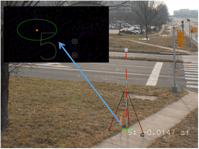
TopoDOT® Measurement of Control Coordinate to Point Cloud Elevation
For civil construction projects requiring location of expansion joints, saw cut lines, or similar features, supplemental analysis of point cloud horizontal accuracy might be required. It is often impractical to place control survey points along vertical surfaces within a typical transportation corridor. In such cases TopoDOT offers practical alternatives to assessment of the horizontal placement accuracy of the point cloud against survey control features.
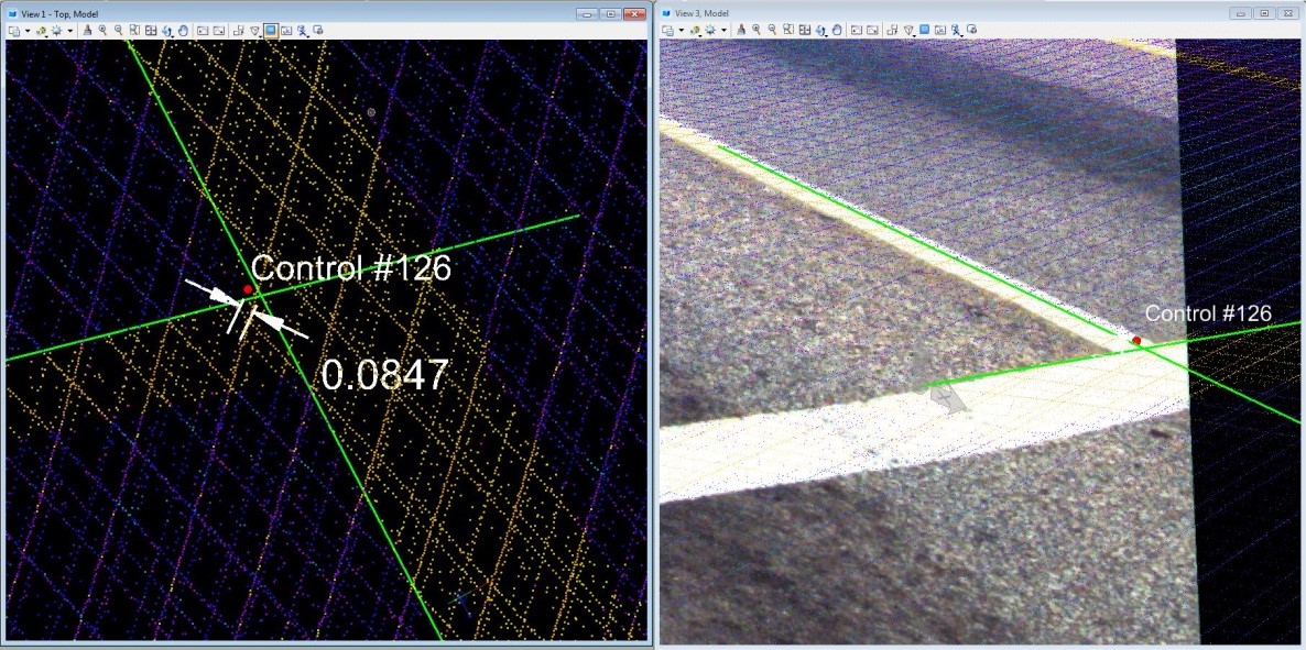
In this first example illustrated below, the control coordinate is measured at the distinctly identifiable intersection of two white paint road lines. Within TopoDOT® it is very easy to extract the intersection point accurately by modeling the edge of each line—in this case simply extracting a long polyline at each line edge in the point cloud. Thus the horizontal distance of the control coordinate from the line intersection can be accurately measured and divided into NE components if necessary.
Of course in this example, the same control coordinate elevation can be compared against the point cloud automatically. Full automation of this process for horizontal measurement is however not sufficiently reliable. That being said, this process only requires less than 1 minute per coordinate.
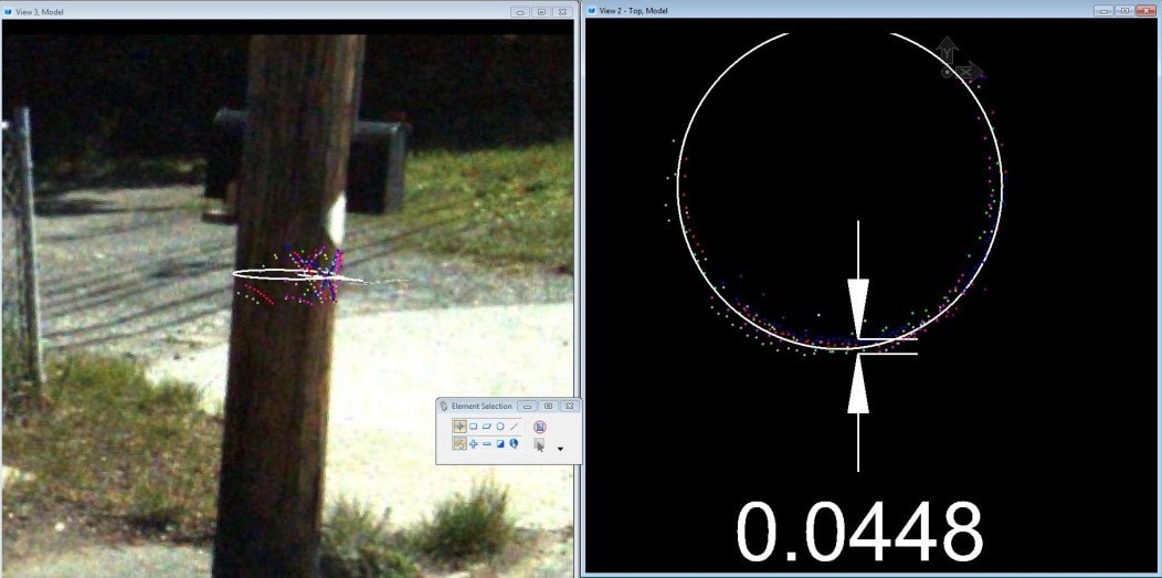
Another reliable source of horizontal alignment evaluation is the comparison of two or more overlapping point clouds along a vertical surface. While there might be no direct local comparison to a survey control coordinate, the relative vertical alignment accuracy is well correlated with absolute horizontal accuracy. Simply stated, it is extremely improbable for deviations in horizontal position of overlapping point clouds to “not” result in corresponding misalignments of point clouds along static vertical surfaces. Such an analysis is also quickly performed in TopoDOT® as illustrated below.
Given the two slightly different approaches for general and topography applications, there are two suggested texts provided for articulating the Survey Control Alignment within a RFP.
Survey Control Alignment RFP Requirement (Static LiDAR General)
The Consultant shall submit to the Customer a plan for a survey control network to be used as a reference to process LiDAR data. The Consultant shall make these control coordinates available to the Customer along with all relevant documentation. Each control coordinate shall be marked, identified and placed such that a sphere of radius “(R)” centered at the coordinate shall contain a clearly identifiable relatively flat hard surface. These coordinates should be selected such that the close proximity surfaces are oriented in different directions.
The distance from the control coordinate to a plane fit to the close proximity point cloud surface shall be evaluated. A summary report shall be given listing all distances, average distance and statistical deviation. 67% of the distances shall be within “(E)” of the plane contained within the sphere, 95% shall be within “2(E)” and 99.7% shall be within “3(E)”.
The Customer at his discretion may add additional survey reference control coordinates to the network unknown to the Consultant for use in the Survey Control Alignment assessment process.
Should any portion of the Survey Control Alignment fail to meet requirements, the Customer shall cooperate with the Consultant by allowing further time to reprocess the data over the area(s) in question and/or develop a strategy acceptable to the Customer to address such anomalies in a way that meets project requirements.
In the event that reprocessing the data is unsuccessful in resolving the anomaly and no alternative strategy can be implemented, the Customer reserves the right to refuse that portion of the data in question providing that this data is within P% of the total. Should data not meeting these requirements exceed “(P)”%, the Customer may at his/her discretion refuse all data or any portion thereof pro-rating payments for services accordingly.
Survey Control Alignment RFP Requirement (Static LiDAR Topography)
The Consultant shall submit to the Customer a plan for a survey control network to be used as a reference to process LiDAR data. The Consultant shall make these control coordinates available to the Customer along with all relevant documentation. Each control coordinate shall be marked, identified and placed such that a circle of radius “(r)” centered at the coordinate shall contain a clearly identifiable relatively flat hard horizontal surface.
The requirements on a survey coordinate location for evaluation of elevation are such that the average of the point cloud data elevations within a circle of “(r)” radius centered at the North/Easting location of the control coordinate shall be expected to be at the same elevation as the control system coordinate.
Should the survey control coordinates be employed for Northing/Easting (NE) evaluation in addition to elevation, the coordinate shall be located at a feature clearly recognizable in the point cloud data such that deviations in horizontal NE position can be accurately extracted and measured. Examples of such features would include: tip of painted chevron, intersection of existing lane lines, or similar features.
The average point cloud elevation within each circle shall be evaluated and compared to the corresponding control coordinate elevation. Of all evaluated control network coordinates 67% shall be within “(Els)” of the average point cloud data elevations contained within the circle, 95% shall be within “(2Els)” and 99.7% shall be within “(3Els)”.
When applicable, the NE location within the point cloud of an identified feature such as a chevron tip or line intersection shall be modeled, extracted and compared to the NE location of the corresponding control coordinate. Of all evaluated control network coordinates 67% shall be within “(NEs)” of the extracted feature location, 95% shall be within “(2NEs)” and 99.7% shall be within “(3NEs)”.
The Customer at his/her discretion may add additional survey reference control coordinates to the network unknown to the Consultant for use in the Survey Control Alignment assessment process.
Should any portion of the Survey Control Alignment fail to meet requirements, the Customer shall cooperate with the Consultant by allowing further time to reprocess the data over the area(s) in question and/or develop a strategy acceptable to the Customer to address such anomalies in a way that meets project requirements. In the event that reprocessing the data and no alternative strategy can be implemented, the Customer reserves the right to refuse that portion of the data in question providing that this data is within (P)% of the total. Should data not meeting these requirements exceed (P)%, the Customer may at his/her discretion refuse all data or any portion thereof pro-rating payments for services accordingly.
For general applications, the value for deviation of the survey coordinate to the nearest plane, “(Es)”, should be chosen such that the extracted features, measurements and model will meet project requirements. Similarly for topography applications, the values for “(Els)” shall be chosen for elevation measurements meeting project requirements and “(NEs)” for meeting northing/easting requirements. It is not unusual for “(Els)” and “(NEs)” to be different values for topography requirements.
As a reference, modern static LiDAR systems employed in support of very high precision AEC projects in plant, piping or similar applications would be expected to meet “(Es)” values of 0.015 foot (4.5mm) in small confined areas. In such areas, the control values are typically acquired with a total station often without need for performing a survey traverse. Thus these requirements are quite tight.
In contrast, static LiDAR data supporting longer range topographic applications might require an “(Els)” value of about .03 foot (9mm) for deviations in elevation and “(NEs)” value of about 0.05 foot. Often the elevation measurements are acquired using a closed level run while northing/easting might be more loosely acquired through GPS RTK methods. The requirements thus reflect the expected value of the control survey coordinate uncertainty in each application.
The value of “P” in this requirement is relatively subjective. In Certainty 3D’s experience, static LiDAR projects often meet requirements completely. However a misaligned scan position or other anomaly is not uncommon. The data from such scans would require reprocessing by the Consultant and/or agreement with the Customer on a strategy for using the data in this area. This is practical if “P” is a relatively small percentage of the entire project. Should misaligned scans exceed say 2% of the total number of scans, one might choose to question the Consultant’s processing procedures, technology, and/or experience. So “P” at about 3-4% might be the limit beyond which the Customer might consider deviations to be excessive and not accept the project.
Finally, as noted in the preceding discussion, it is not uncommon for some topographic applications to assess only elevation alignment to survey coordinates and leave northing/easting position to be assessed from overlapping point cloud alignment. This approach is often successful with requirements addressed in Step 2.
Step 2: Scan to Scan Alignment
Individual point clouds acquired at each scan position can be considered to be rigid bodies. One might envision the individual scans as being pieced together like a puzzle whereby collectively they describe the entire scene. How they fit together, i.e. their respective position and orientation, is primarily determined through reference to external control reference targets described in Step 1.
However a good result in Step 1 is not conclusive of correct data alignment. Keep in mind that the scanner has only located the reference targets, which is an incomplete assessment of its performance in acquiring the arbitrary surfaces across the scene. For example, the scanner performance might be optimized for identifying and locating these “cooperative” targets but may show poorer performance to arbitrary surfaces of widely varying reflectivity. In addition, process mistakes such as misalignment of vertical rods over survey nails, misidentification of reference targets or blunders in the control survey coordinate itself might still show acceptable results in Step 1, yet result in significant misalignments of point cloud data. Thus Step 2 focuses primarily on overall data alignment.
A simple process executed in TopoDOT® can be quickly applied to areas with overlapping point cloud data from two or more individual scan positions. Begin by opening the relevant scan positions in TopoDOT® and identifying each by color. Inside a room, for example, select cross section data across areas with common point cloud data. Select cross sections with varying directions from the floor, ceilings and walls. In each case TopoDOT® automatically provides an orthogonal cross section view of the overlapping point cloud cross-section for easy analysis and measurement.
For outdoor topography applications, select cross sections of data between adjacent scan positions and follow the same process. In the TopoDOT® image below, each point cloud is identified by color. A cross section of data within the fence will be automatically shown in another view orthogonal to the cross-section plane. Vertical misalignments can be easily identified and measured. Note that several scans can be evaluated quickly by selecting a cross-section in an area with more than two overlapping scan position points (colors). In the scene below, an additional cross-section analysis in the same area oriented orthogonally would typically be sufficient to evaluate the alignment of these four positions. Should a misalignment appear, further inspection will quickly identify the misaligned scan position(s).
Horizontal alignment can be evaluated through horizontal cross-sections of vertical surfaces such as building walls or poles. In the following TopoDOT® image, a horizontal cross-section of point cloud data was selected. Again TopoDOT® automatically provides the orthogonal view of the data cross-section. A quick analysis shows tight alignment at the corner of the building and thus tight horizontal relative orientation between the two scan positions.
One might expect the potential for automation of this alignment evaluation by some automated comparison between point clouds. However such automation over the entire cloud requires significant processing time, often resulting in anomalies requiring further inspection using the same process as the selective cross-section approach described herein. Alignment evaluation of two adjacent scans using the cross section technique might only take 10-20 seconds and is easily learned and interpreted. Thus in Certainty 3D’s experience, further automation would bring no real productivity or accuracy benefit.
An example of how one might formulate the alignment requirement for static LiDAR data in an RFP is shown below.
Scan Alignment RFP Requirement (Static LiDAR data)
The misalignment of individual point clouds covering common areas acquired at scan positions in close proximity shall not exceed “(Es)”. The point cloud data evaluated will be restricted to a radial distance of “(R)” from the center of each scan position.
The Customer will evaluate alignment by selecting cross sections of point cloud data and measuring the separation between individual point clouds. Separation shall be defined as the shortest distance between two or more lines best fit to points from each individual scan within the cross-section plane. When overlapping data from more than two scan positions is present and all data is within the radial distance “(R)” from each respective scan position center, then the distance between each pair of individual scan position data shall be measured.
The Customer will typically select two or three cross sections within each area of common data between two or more individual point clouds. Any differences exceeding “(Es)” shall be documented and provided to the Consultant. The Consultant shall have the opportunity to adjust the data, document the adjustment along with comments on the cause of the misalignment. Any adjustment and/or acceptable strategy to utilize the data must be provided to the satisfaction of the Customer assuring that overall project objectives are met.
Should the Consultant fail to provide adjustment(s) and/or strategies acceptable to the Customer, the Customer shall at his/her discretion require individual scan(s) to be repeated employing established control to replace that data. Should the number of misaligned scan positions exceed “(P%)” of the total number of scan positions, the Customer may refuse all data or any portion thereof prorating payment to the percent of scans accepted.
The value of “(Es)” shall vary in accordance with the nature of a project and its ultimate objectives. For example, pipe fitting applications might require and “(Es)” value of approximately 0.005 feet (1.5 mm). In contrast, large area topography applications along a transportation corridor would typically choose an “(Es)” value of about 0.03 feet (9mm).
The requirement on a distance “(R)” is especially relevant to longer range topography applications as there is some degradation of the data over long distances and/or shallow angles between the scanner laser beam and a surface. Typically, for tripod mounted operations, one might set the limits on “(R)” at approximately 80 feet as data along a horizontal surface will become less reliable at these shallow angles.
Steps 1 and 2 collectively establish a traceable lineage from the point cloud data to the control survey coordinates for static LiDAR data. The methods presented are intuitive, produce quantifiable metrics and are relatively quick to implement. In the next section, we examine a similar process applied to mobile LiDAR data.
Mobile LiDAR Data
TopoDOT® offers tools and a relatively simple two-step process to establish lineage between the mobile LiDAR data point cloud and survey control coordinates. In contrast to static LiDAR data, the following two step process is effectively reversed in order Interestingly the structure of mobile LiDAR lends itself more readily to a relatively complete automation of alignment assessment. Once again, these processes yield quantifiable and easily understood metrics that are “continuous” along the entire corridor.
Step 1: Flightline Data Alignment
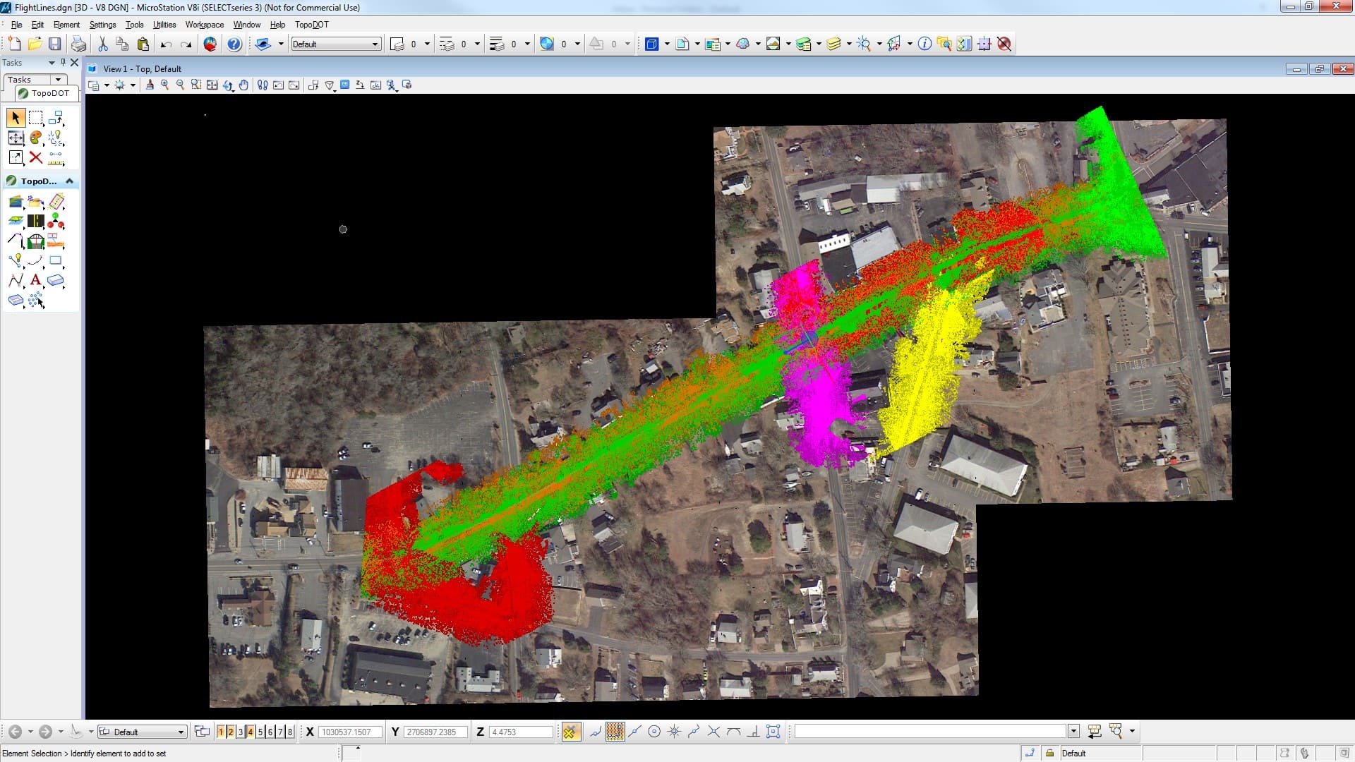
“Flightlines” refer to mobile and aiborne data associated with individual flight or driven trajectories. Typically each Flightline covers a single “pass” along the corridor. If the corridor is very long, the data may be divided up into separate Flightlines just to limit the amount of data in a file. Note that such a Flightline data is commonly exported in the LAS format. Within the LAS format, there is a “point source ID” identifier. The point source ID facilitates easy association of points to a specific source Flightline trajectory.
The alignment of overlapping multiple Flightline data sets along a corridor is in itself a form of survey control. This statement is based on the two following premises:
1) Each stationary surface in the scanned area is a reference.
2) Mobile LiDAR systems rarely deviate from the “true” trajectory at the same place, in the same way, at different times.
The first premise states that individual Flightline point clouds over a common static surface should be tightly aligned within an acceptable tolerance. Thus static objects such as road surfaces, poles, curbs, and break lines serve as a “relative” form of reference control between overlapping point clouds associated with each Flightline.
The second premise leads one to conclude that any misalignment between two Flightlines will be indicative of a deviation of one or both trajectories associated with each Flightline. Conversely, well aligned Flightlines are indicative of high quality trajectories and good data quality. These premises lead to the conclusion that Flightlines tightly aligned within some tolerance serve as an excellent indicator of data quality “continuously” along a corridor.
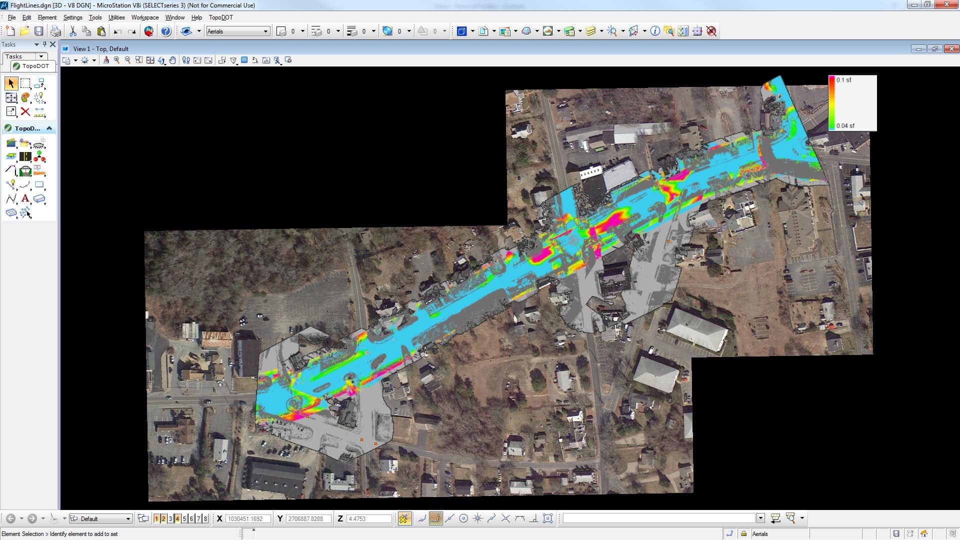
TopoDOT® offers the Flightline assessment tool to automatically compare overlapping point cloud data acquired along different trajectories. The result is a raster image color-coded according to the maximum distance between Flightlines. In the example below, light blue indicates a misalignment distance within 0.04 feet. Green to red color gradients indicate increasing deviations from 0.04 to greater than 0.1 feet. Thus Flightline misalignments are easily identified and located.
An example of how one might formulate a Flightline alignment requirement (mobile LiDAR data) in an RFP is given below:
Flightline Alignment RFP Requirement (Mobile LiDAR Data)
Mobile LiDAR data acquired over individual passes along the corridor will be identified as Flightlines. Typically a Flightline data set is comprised of the point cloud and image data acquired over a “single” trajectory in one direction along an individual road or highway.
Individual Flightline data shall be identified through the “point source ID” in its LAS data file. Long trajectories exceeding “(M)” miles along a continuous roadway should be divided up into individual Flightlines in order to maintain manageable file sizes.
The Consultant shall acquire at least two Flightlines along each corridor. The trajectories need not be in the same lane, but they should have significant common areas of data especially along the hard surfaces. Alignment deviations between these Flightlines shall not exceed “(Ef)”.
The Customer may at his/her discretion return to the Consultant any data exceeding these alignment tolerances for additional processing to adjust the data. Any returned data shall be accompanied by a report indicating the source of the misalignment and how the deviation was resolved. Should such additional processing prove unduly time consuming, the Customer may, at his/her discretion, accept identification of the more accurate Flightline using local control survey data as a comparison assuming the selected Flightline alone is adequate to meet project Coverage requirements.
Construction quality topographies extracted from mobile LiDAR data will typically use a value of about 0.05 foot (15mm) for “(Ef)” above. TopoDOT® offers two automatic tools for assessing this alignment in the vertical direction over hard surfaces. Evaluation of Flightline alignment is generally limited to hard surfaces as areas containing vegetation or other high noise data yield results which are difficult to interpret.
For project requirements less demanding of spatial accuracy, such as asset identification and location, the relaxation of requirements should not become excessive. Misaligned Flightlines can confuse algorithms attempting to automatically identify, locate and extract features as well as the technicians processing the data. For those reasons, we’d recommend Flightline misalignment not exceed say 0.1 to 0.15 feet for such applications. Finally, a typical value for “M” might be > 3 miles (5km).
Step 2: Survey Control Alignment
Having established the “relative” data alignment quality in Step 1, Step 2 compares the point cloud to Control survey coordinates. TopoDOT®’s “Point Cloud to Data Analysis” tool performs this analysis automatically as described in the preceding Static LiDAR Data section. The only difference is that typically the control coordinates are identified with a mark on the roadway surface, a painted chevron for example, and there is no reference target placed over it. As discussed in the static LiDAR section, these markings can be modeled and compared against a control survey coordinate in northing/easting as well as elevation.
Collectively, Steps 1 and 2 establish a traceable and continuous lineage complete with quantifiable metrics between the point cloud and the control survey coordinates along the entire corridor. Note that survey control points should be placed on hard surfaces on somewhat flat areas where the average point cloud elevation within a radius of about 0.5 feet (15cm) should equal the control coordinate elevation.
As the Survey Control Alignment and Flightline Alignment requirements are complimentary for mobile LiDAR data, the following example formulation of a Survey Control Alignment requirement in an RFP contains references to both.
Survey Control Alignment RFP Requirement (Mobile LiDAR data)
The Consultant shall submit to the Customer a plan for a survey control network to be used as a reference to process LiDAR data. The Consultant shall make these control coordinates available to the customer along with all relevant documentation.
Each control point shall be marked, identified and placed at some relatively flat hard surface location. The requirements on this location are such that the average of the point cloud data elevations within a circle of “(r)” radius centered at the North/Easting location of the control coordinate shall be expected to be at the same elevation as the control system coordinate.
The average point cloud elevation within each circle shall be evaluated and compared to the corresponding control coordinate elevation. Of all evaluated control network coordinates 67% shall be within “(Elm)” of the average point cloud data elevations contained within the circle, 95% shall be within “(2Elm)” and 99.7% shall be within “(3Elm)”.
When applicable, the N/E location within the point cloud of an identified feature such as a chevron tip or line intersection shall be modeled, extracted and compared to the N/E location of the corresponding control coordinate. Of all evaluated control network coordinates 67% shall be within “(N/Em)” of the extracted feature location, 95% shall be within “(2N/Em)” and 99.7% shall be within “(3NEm)”.
The Customer may at his/her discretion add additional survey reference control coordinates to the network unknown to the Consultant for use in the Survey Control Alignment assessment process.
Note that for LiDAR data acquired by mobile LiDAR systems, the data shall first meet Flightline alignment requirements prior to Survey Control Alignment evaluation. Should areas of the data fail to meet Flightline alignment requirements, they will be identified and documented. In cases where misaligned Flightlines include the circular area employed in the evaluation of point cloud data elevation at a survey control point, their effect on the survey control analysis results should be documented.
Should any portion of the mobile LiDAR data fail to meet Flightline Alignment and/or Survey Control Alignment, the Customer shall cooperate with the Consultant by allowing further time to reprocess the data over the area(s) in question and/or develop a strategy acceptable to the Customer to address such anomalies in a way that meets the project requirements.
In the event that reprocessed data fails to meet these requirements and no alternative strategy can be implemented, the Customer reserves the right to refuse that portion of the data in question providing that this data is within “(P%)” of the total. Should data not meeting these requirements exceed “(P%)”, the customer may at his/her discretion refuse all data or any portion thereof pro-rating payments for services accordingly.
The values for “(Elm)” and “(N/Em)” should be chosen such that the extracted features, measurements and model will meet project requirements. As a reference, modern mobile LiDAR systems employed in support of roadway construction projects would be expected to meet “(Elm)” and “(N/Em)” values of 0.05 ft (15mm). Thus 67% of all elevation comparisons to survey coordinate data would be within 0.05’, 95% within 0.1’ and 99.7% within 0.15’. For planning, GIS and other applications, the value of “(Elm)” and “(N/Em)” might be significantly larger.
The value of “(P)” in this requirement is relatively subjective. In Certainty 3D’s experience, practically every high accuracy mobile LiDAR project will show some area deviating from Flightline Alignment and/or Survey Control Alignment requirements. These two tests will serve to identify and isolate such areas. Such areas would require reprocessing by the Consultant and/or agreement with the Customer on a strategy for using data in this area. This would be practical if “(P)” is a relatively small percentage of the entire project. However should these areas exceed say 25% of the project, one might chose to question the Consultant’s processing procedures, technology, and/or experience. So “(P)” at about 20% might be the limit beyond which the Customer might consider deviations to be excessive and not accept the project.
This process has been tested and proven on hundreds of LiDAR data projects. For more detail and live demonstration of this process, please contact Certainty 3D directly.
Calibrated Image Alignment
Calibrated images are quickly becoming a key component of LiDAR data. The synergy between the point clouds and calibrated images is significant and increases greatly with the quality of the image calibration. Certainty 3D has repeatedly demonstrated that “well calibrated” images can improve TopoDOT® 3D model extraction productivity by about 30%, while enhancing the quality of the extracted 3D model and reducing much of the tedium associated with the extraction process.
If calibrated images are to be included as part of the delivered LiDAR data set there should be clear requirements placed on these images within the RFP. The required information associated with a calibrated image is relatively well-known using standard photogrammetry principles. Specifically, each image should have metadata attached to it describing the:
- Camera Models
- Image Location (project coordinate reference frame)
- Image Orientation (project coordinate reference frame)
- Image file ID and metadata
Certainty 3D website’s TechNote section offers TechNote #1009, “TopoDOT® Open Calibrated Image File Format V2” for direct calibrated image import into TopoDOT®. This format is simple, open and non-proprietary. You can find this document on the C3D University web page or hyperlink from the nearby image.
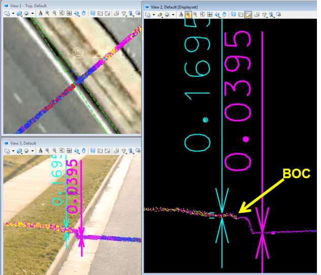
Image/point cloud alignment can be easily assessed within TopoDOT® by comparing a line feature accurately extracted from the point cloud to the corresponding identified edge in the calibrated image. The process begins by extracting vectors from the point cloud alone. These vectors should be easily identified in the image such as the corner of a building, the line in a road or the edge of a sign. Then import the calibrated image into the scene. TopoDOT® will automatically map the line work to the same perspective view as the image. Compare the line work extracted from the point cloud to the corresponding edge in the image. Zooming into the edge, one can count the amount of pixel offset. Repeating this process using edges oriented along different directions will give a good indication of the camera calibration quality.
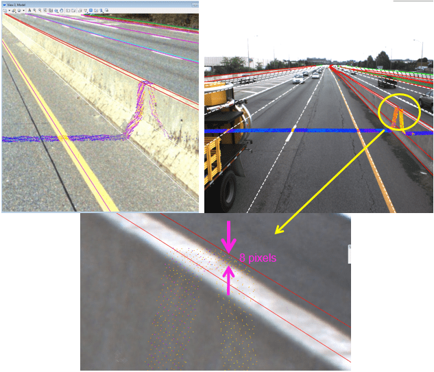
In the above examples, the left image is precisely aligned to within 1 pixel. The image on the right, from another project and LiDAR system, is misaligned by about 8 pixels. The number of pixels is determined by simply zooming in and counting the pixels.
It should be noted that not every image in a mobile LiDAR data set must be inspected individually. Any camera misalignment will typically be consistent throughout the project. The challenge is to quickly review thousands of images in order to identify a misalignment. TopoDOT®’s Visual Inspector tool addresses this challenge by allowing the user to quickly inspect thousands of images along a corridor project.
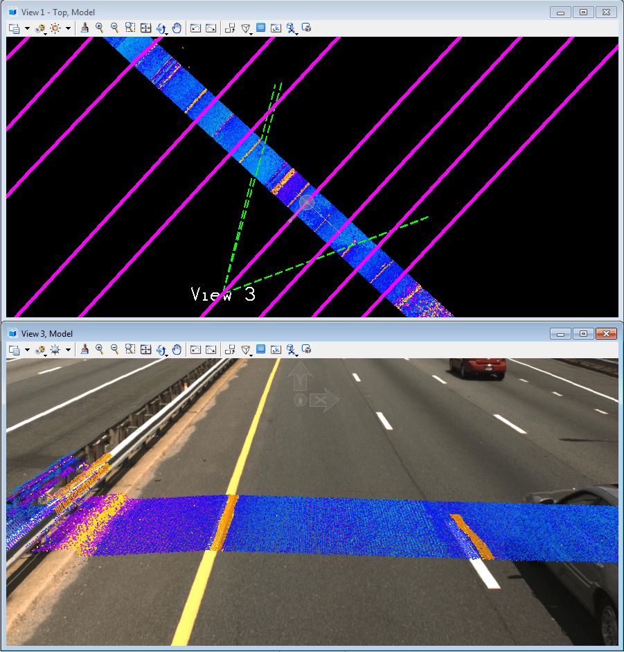
As illustrated below, TopoDOT®’s Visual Inspector quickly extracts a trajectory for each individual camera (pink lines). Visual Inspector then steps through each image along that trajectory automatically loading a cross-section of point cloud data at a fixed distance from the camera location. The screenshot below shows a top view with the image vectors in green, the point cloud cross-section and the camera trajectory paths.
The calibrated image is loaded into the second view simultaneously. As there are many common linear features such as stripes, curb edges guard rail, etc. within the image and the point cloud, obvious misalignment is easily noticed. In the following TopoDOT® screenshot, we see camera misalignment between road stripes in the image and point cloud. Once this is noticed, the aforementioned technique of extracting a vector within the point cloud, zooming into the image and counting the pixel offset would be performed for a quantitative result. Note that the process can be further accelerated by examining every tenth image for example since the characteristics of the misalignment will not change over such a short distance.
Calibrated Image Alignment RFP Requirement
The Customer will submit calibrated images acquired by the on-board LiDAR system cameras. In addition to the image files, the following information will be given for each image.
- Camera/Lens model (unique to each camera/lens pair for best results)
- Camera Location (project coordinates for each image)
- Camera Orientation (defined with respect to project reference frame)
Image quality will be consistent with a camera of “(W x H)” pixel array and a lens field of view of “(FOV)” degrees. Images will exhibit appropriate clarity and resolution as would be expected when using appropriate aperture, shutter speed, or equivalent operating parameters.
These images will be used by downstream applications offering the capability to import calibrated images while using this information to map the point cloud and CAD elements to the same perspective view with very high precision. The exported file format is documented in the attached appendix.*
These images shall be sufficiently calibrated such that the alignment to the point cloud data is within “(Px)” pixels. In order to evaluate the alignment, the Customer will extract approximately 20 CAD line elements representing edges in the point cloud. Such CAD elements easily extracted with a high level of precision would be the corner of a building, a road lane line an edge of a sign or similar straight line feature. Edges will be selected such that they are oriented within the image at varying angles such as the vertical corner of a building, a horizontal roof line and a diagonal perspective view of a road line.
The Customer will then measure the alignment by importing calibrated images into an application that will map the CAD elements and point cloud to the same perspective view using information above to accommodate distortion, placement and orientation of the image. The pixel distance from each CAD element edge to the image edge will be recorded at about 20 locations for each camera. The Customer may at his discretion refuse images where edge misalignment with corresponding CAD elements exceeds “(Px)” pixels.
*Note: A separate document defining the detailed calibrated image file format will be several pages long. Since applications such as TopoDOT® offer well documented open data formats, it will typically be easier and more readable to refer the reader to this document.
As is the case with Flightline and Survey Control Alignment, the requirements for image alignment and evaluation do not address system level processes such as camera modeling, calibration and determination of position and orientation of each image. These processes are complex and the responsibility of the Consultant.
One should note that for obvious reasons, static LiDAR images are typically more tightly calibrated and aligned than those of mobile systems. Based on Certainty 3D’s field experience, reasonable values of “(X)” would be about 1 pixel for static system images and 5 pixels for mobile LiDAR system images.
Process Overview
These three alignment evaluations: Image, Scan/Flightline and Control Survey establish a lineage from each LiDAR data component to the reference survey control data as illustrated below.
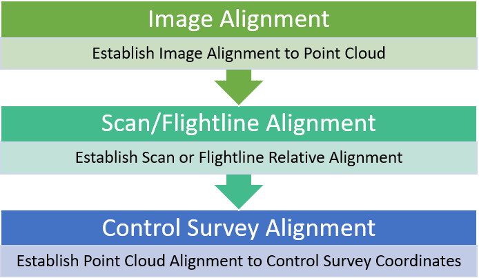
Simply stated, the calibrated images are aligned to the point cloud, individual point cloud Flightlines (mobile)/Scans (static) are aligned to each other and finally the total point cloud is aligned to the reference survey control coordinates. This process thus establishes a clear and traceable lineage from any data component to the reference control survey. Note the control survey is typically the only “sealed” legal document reflecting the accuracy of the data.
It is clear that any alignment not meeting requirements effectively “breaks” the lineage thereby calling into question the spatial orientation of data components preceding the break. So for example a Flightline or Scan alignment not meeting requirements would call into question the orientation of images associated with that Flightline even though these images might meet alignment requirements to the point cloud. Therefore whenever a LiDAR data component is reprocessed to address an alignment anomaly, the upstream data components in the alignment evaluation must also be reprocessed.
Note that Certainty 3D has seen many mobile data sets where initially point cloud data was well-aligned with calibrated images. However the point cloud data was found to not meet Flightline and/or Control Survey alignment requirements. Consultants would often reprocess the point cloud orientation while neglecting to apply the corresponding position changes to the “upstream” calibrated images. Thus, while the reoriented point clouds would then meet alignment requirements, the calibrated images were no longer aligned to the point cloud often to such an extent as to make their use impractical. It is therefore imperative to “completely” reapply the alignment evaluation tools provided in TopoDOT® for every LiDAR data set component following any data adjustment.
LiDAR System Data Characteristics
In the first sections of this document, the data requirements focused primarily on alignment and establishing lineage back to the control survey reference coordinates. The following sections will focus on assuring data characteristics will support feature identification, measurement and model extraction consistent with project requirements.
Establishing Random Noise Requirements for Point Clouds
As explained in the section, “Origins of Data Uncertainty”, every sensor exhibits some level of random uncertainty (noise). Typically random noise manifests itself in a point cloud as “fuzziness”—a thickness over relatively flat surfaces. Such noise is generally random in nature with a bell-shaped distribution about its mean.
The fundamental question to consider in establishing random noise requirements is, “What level of noise contributes to extraction errors exceeding project requirements?” Leaving more rigorous analyses to the academics, we find that as a rule the statistical deviation of the random noise should be about one fourth (1/4) the smallest feature dimension one is attempting to identify within the point cloud.
This concept is demonstrated in the TopoDOT® image. In this case, the feature to be identified is the curb. However upon closer reflection the smallest feature is the grass/curb interface. The peak-to-peak thickness of the point cloud data over the relatively flat surface cement surface is just under 0.04 feet. The thickness of the grass is about 0.17 feet. Thus this “4x Rule” provides point cloud data of high enough resolution to identify the back of curb/grass interface.
The preceding topography example is well-suited to other architecture, engineering, construction (AEC) and similar applications as well. This is especially true when the LiDAR data is comprised of point clouds only without calibrated images. Should calibrated images be included in the LiDAR data, often the levels of random noise and point density (see below) can be lessened.
Random Noise RFP Requirement
The Random Noise Level shall not exceed a peak-to-peak value exceeding “(N)”. Random noise shall be measured by analyzing several representative cross section samples of point cloud data across relatively flat surfaces in the scene.
Flat surfaces are identified as those whose inherent roughness would be at least an order of magnitude less than the peak-to-peak random noise level being measured. In plant, piping, and similar AEC applications demanding a higher precision value of “(N)”, the flat surface might be a bare floor or un-textured wall for example. For outdoor topography applications, flat surfaces would be the small area of a roadway, sidewalk or similar surface.
The Customer will select several flat areas within the point cloud data for analysis. At each area, a cross section of point cloud data will be extracted such that the viewing plane of the data is orthogonal to the cross section plane. The width of the cross section shall be sufficiently narrow such that any curvature of the surface over the width of the cross section will have an insignificant contribution to the peak-to-peak data value. The peak-to-peak width of the data will be measured and compared to “(N)” at each location.
Should the peak-to-peak values consistently and significantly exceed “(N)”, the Customer may at his/her discretion refuse acceptance of the data.
Given Certainty 3D’s experience processing hundreds of transportation corridor topography projects, a peak-to-peak random noise level of 0.04 foot (+/-0.02 foot or +/-6mm) is recommended for accurate feature extraction. Note that this level of random noise is well within the performance level of many modern laser scanners designed for this purpose. Other applications demanding higher precision might require a lower level of random noise. In such cases the 4x rule will prove sufficient in determining the appropriate level of random noise.
This requirement allows the Customer some discretion in accepting the random noise level. In Certainty 3D’s experience, it would be unreasonable to refuse topographic point cloud data because somewhere in the scene the peak-to-peak noise was 0.05 foot or even 0.06 feet. However, for example, consistent noise levels exceeding 0.1 foot might negatively affect accurate identification of smaller features in the scene and thus may not be acceptable.
Point Density
Point cloud density is a critical data characteristic. The correct density for a particular project depends roughly on the size of the smallest feature to be extracted. More specifically, the surface area of the feature must be sampled at a sufficiently high density such that this feature may be extracted to an accuracy meeting project requirements.
The appropriate point cloud density depends on the geometrical structural cues of the feature as well as the techniques employed in identifying and extracting the feature from the LiDAR data. For example, techniques which depend on selecting individual points from the point cloud require far higher density than tools designed to exploit the linear structure of typical features. It should also be noted that high resolution calibrated images mapped to a point cloud coordinate system are synergistic in nature and lessen the density requirements on the point cloud. For these reasons, a rigorous analysis for calculating the point density can become rather complex.
Consider an indoor AEC application requiring feature extraction with high precision, say on the order of 0.006 feet (2mm). If the software extraction is dependent on selecting just the nearest data point of a point cloud, it would imply that the point cloud spacing must be about 0.006 feet (2mm). Extrapolating this requirement over 1 square foot the point density would be over 30,000/square foot. Clearly this leads to an enormous amount of points per scan position and inefficiencies in downstream processing workflows due to the volume of data.
Such an approach is typically confined to small area indoor AEC applications. Such high point cloud densities produce extremely large data files thus placing high demands on computer memory and data storage. Often these large data files will have negative effects overall processing productivity.
Since some topography extraction methods are focused on selecting a data point, they too require point spacing sufficiently dense to meet say a 0.03 feet (9mm) requirement. This would require a point cloud density exceeding 1000 points per square foot. Such densities are extremely difficult to acquire in a cost effective and efficient manner along typical road topography applications for example. Moreover these large amounts of data result in the same negative impact on computer memory, data storage and processing productivity.
Given Certainty 3D’s experience in processing hundreds of successful topography projects, we will provide a practical level of point cloud density requirements designed to achieve a balance between current LiDAR technology performance, maximum field productivity and cost in this application area. Since TopoDOT® makes full used of the linear structure of topographic features, efficient modeling tools and full use of calibrated images when available, the point cloud densities required by TopoDOT® processing workflows are significantly lower than those cited above.
A suggested text for Point Cloud density requirement inclusion in an RFP is given below:
Point Cloud Density RFP Requirement
The Point Cloud Density acquired by the Static LiDAR System shall be greater than “(D)”. Point Cloud Density shall be measured by sampling representative areas of point cloud data along the project. Reasonable exceptions with respect to diminished or non-sampled areas occurring as a result of scanner obscured lines of sight will be given at the Customer’s discretion. Should the point cloud density be less than “(D)” with no reasonably unavoidable blocked lines of sight present, the Customer shall at his/her discretion require additional data be acquired or refuse acceptance of the data.
Complex analyses aside, employing TopoDOT® one can set point cloud density requirements at the following approximate levels to achieve expected construction quality topography detail as:
| System Platform | Minimum Density |
| Airborne | >5 points/sq ft (>45 points/sq m) |
| Mobile | >20 points/sq ft (>180 points/sq m) |
| Static | >20 points/sq ft (>180 points/sq m) |
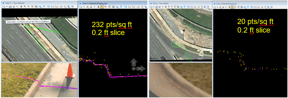
Note in the example of curb extraction above, equal width cross-sections of data are shown at 232 points/square foot and 20 points/square foot. Employing the profile extraction tools provided in TopoDOT® the curb line can be extracted from both point cloud densities. However Certainty 3D has empirically determined the 20 points/square foot density level to be the “approximate” minimum for static LiDAR platforms whereby accurate extraction of curb lines is practical and acquisition costs are reasonable.
The above density requirements are also tempered with the practical performance of each platform. For example, we would not expect to extract the same level of detail from airborne LiDAR data at just 5 points/square foot as we would with mobile and static data. However achieving that extra density from airborne data could be costly. So Certainty 3D has found these density levels to yield very useable models from airborne LiDAR data yet still be acquired at a reasonable cost.
Similarly the minimum density levels for mobile and static LiDAR platforms are practical with respect to current system performance and reasonable acquisition costs. Certainty 3D has found that topographic models meeting or exceeding typical transportation corridor requirements can be extracted at each point cloud density level. These respective density levels for each system reflect a practical field application of current technology with no undue burden of additional cost and/or schedule.
TopoDOT® offers two tools for measuring point cloud density. The first, “Point Density Overview” exports an image file with color codes corresponding to point cloud density project. Green area exceeds, yellow slightly exceeds and red areas are below minimum density.
For static LiDAR data (tripod), it is not uncommon for point cloud density to vary quite dramatically across the scene since point density diminishes rapidly as a function of distance from the scanner. Thus lower densities between scan setup positions are typical. Should the scanner operator place setups too far apart—often to save time—the density between adjacent positions can become significantly lower than requirements. Thus it is typically good practice to validate density halfway between scan positions.
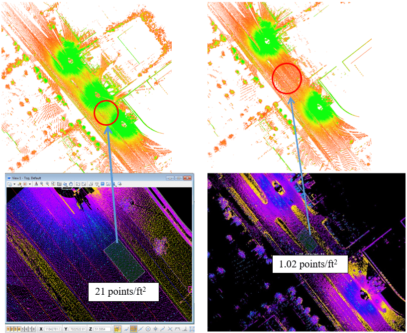
Consider the following example of static LiDAR data first analyzed with TopoDOT®’s Point Cloud Density Overview tool. In the original data the left image illustrates three scan positions optimally spaced for coverage of lanes running northwest. In the right image, the center scan data was unloaded to simulate scans placed too far apart. This area is now predominately red.
Further analysis of this area using TopoDOT®’s “Point Cloud Density” tool is shown beneath the two color coded images. The exact point cloud density is shown within a “fence” placed at locations between scans for precise measurement. The points counted in the left optimally scanned image show just over 20 points per square foot. Contrast this density with that of the right image where one scan has been removed. The density between the scans is now only 1 point per square foot and well below the requirement.
To summarize, TopoDOT®’s Point Cloud Overview tool is used for a quick assessment of the point cloud density across the entire project in the form of a color-coded image. Those areas coded red for low density can then be assessed directly in the point cloud using TopoDOT®’s Point Cloud Density tool for a very accurate density evaluation and comparison to requirements.
Once again the RFP requirement gives discretion to the Customer to refuse or accept the data. It might not be reasonable to refuse data if say density fell to say 16 points per square foot in some isolated area. However for a static LiDAR project, one could reasonably refuse data falling significantly “and” consistently below the minimum density level as being substandard and incorrectly acquired.
In contrast to static LiDAR point cloud data, the point cloud density “structure” generated by mobile LiDAR systems is typically more consistent, especially over areas in close proximity to the vehicle path. Mobile LiDAR system performance parameters of scanner measurement and line rate are generally fixed. Thus density primarily changes as an inverse function of vehicle speed, i.e. density decreases with increased speed. So for constant speeds the point cloud density will stay reasonably consistent.
An example of mobile LiDAR data acquired with a single-scanner oriented about 45 degrees to the roadway is shown below. Each solid line is actually comprised of very closely spaced individual points generated as the mirror rotates through a single line. The next rotation of the mirror generates a seemingly parallel line with significantly more spacing. The reason for this pattern is that the mirrors cannot physically rotate quickly enough to space out the individual points along a line and close the gap between subsequent lines. Note that dual scanner systems are not uncommon and will result in an additional set of lines oriented about 90 degrees to each other.
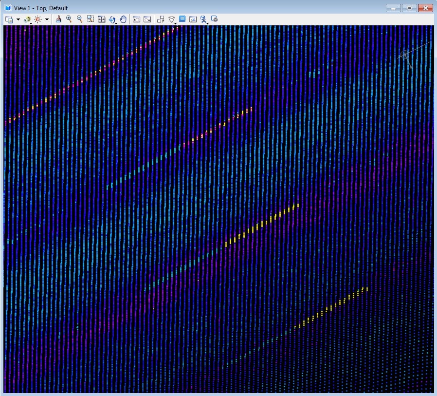
The consistency of the point density provided by mobile systems generally degrades rapidly with distance from the vehicle toward the sides of the corridor. This is generally a consequence of geometry as the laser beam incident angle to the topography surface becomes shallow.
“Shadowing” is caused by a fixed object along the corridor blocking the beam thus leaving a shadow wherein the point cloud density is greatly diminished or missing altogether. Such obstacles would be barriers, trees or signs. The occurrence of shadowing was the motivation for the reference to “reasonable exceptions . . . as a result of scanner blocked lines of sight. . .” within the RFP text. The interpretation of “reasonable exceptions” is broad as in certain instances shadowing is unavoidable, yet in others significant shadowing can be avoided with proper scanning methods and processes.
Consider first a case of “unavoidable” shadowing within mobile LiDAR data. Certain objects might simply block the scanner line of sight creating a shadow with limited or no point cloud data. While an operator using a static type platform (tripod or TopoLIFT™) might be expected to situate the scanner at different positions within the scene to effectively “fill in” such shadows when reasonably possible, one should recognize a mobile LiDAR system does not offer that same level of flexibility. For example, a guard rail on the side of the road will effectively block the scanner line-of-sight to the surface behind it resulting in an area with no point cloud data or a “shadow”. One cannot reasonably expect the mobile system to fill in such areas as its trajectory is obviously confined to the roadway. Thus the Customer shall understand and apply reasonable exceptions when evaluating the data.
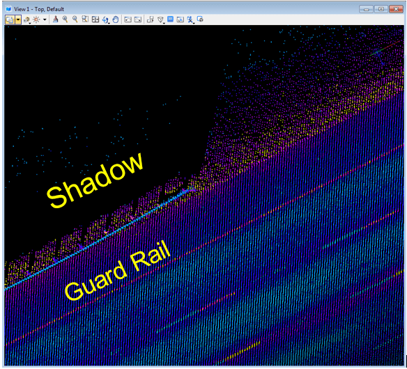
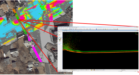
The preceding image illustrates the occurrence of shadowing within a mobile LiDAR data point cloud. From the top view, the roadway is clearly evident. The blue line off the side of the road is actually a guard rail. While the surface of the guard rail is well described by the point cloud data, the “shadow” behind it is dark and practically devoid of points. Such shadows are to be expected in mobile LiDAR data and these areas should not be subject to the general point cloud density requirements.
Contrast this case with an “avoidable” case of traffic shadows in the mobile LiDAR data shown below. In this case shadowing is caused by two moving vehicles blocking the scanners line of sight. One should expect a single Flightline to exhibit such shadows as traffic will always be present. However recall that the Flightline Alignment requirement calls for at least two Flightlines be acquired with overlapping data along the same corridor. Thus in addition to providing valuable alignment information, multiple Flightlines will typically “fill in” traffic shadows as vehicles will not be at the same place at different times.
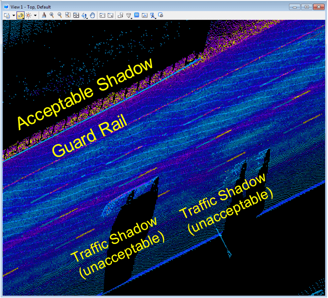
Note that traffic shadows can also be largely avoided through intelligent planning and proper scanning techniques. For example, data acquisition during off-peak traffic times is very helpful. Common sense techniques such as avoiding driving next to a vehicle in a parallel lane for extended periods will also avoid excessive traffic shadows. Thus while some isolated traffic shadow might be acceptable, the Customer should consider not accepting data with excessive traffic shadowing.
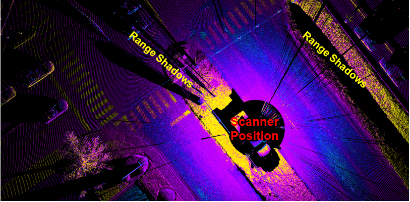
Shadows within static LiDAR system data have a different structure than mobile. That is to be expected since the beam rotates about a vertical axis at its scan position thereby generating shadows emanating radially from the scan position center. As shown below from the top view of this static LiDAR data, obstacles blocking the scanner field of view result in range shadows behind them. Good field practices and scanning techniques will assure that other scan positions be located such that the additional data will “fill in” these shadows. Unless there is no practical means of locating the system in an appropriate position, such shadows should generally not be acceptable. Excessive shadowing that could have been avoided through properly placed positions might indicate substandard field techniques. A Customer might at his discretion refuse such data especially if such shadows are in areas of importance to meeting overall project requirements.
Airborne LiDAR systems function fundamentally the same as mobile terrestrial LiDAR systems. That is to say they generate point clouds as a single axis rotating laser scanner moves along a trajectory measured by GPS, IMUs and computer processors. Point density is again inversely related to flight speed. LiDAR scan density might vary from a single point or two per square meter to several tens of points per square meter. This document calls for a density requirement of 45+ points per square meter as the primary application is detailed corridor mapping. Typically rather small features such as curb lines are accurately extracted from such data.
Keep in mind that this point density for airborne data is admittedly on the high end of available data and offered as a reference. Lower density point clouds are useful for corridor mapping if the extracted models support project requirements. In fact such data is typically very useful when supplementing very high density data acquired by mobile LiDAR systems along a corridor as the airborne data provides topography information well beyond the practical range limits of the mobile LiDAR data. It should be noted that the LiDAR data requirements will differ between the respective areas of terrestrial mobile and airborne LiDAR data. Also extraction will not be as detailed over areas of lower point density.
In addition to shadowing effects, one should understand that certain site conditions will result in areas of no data at all or “less useful” data. Water filled puddles for example will generally result in missing or distorted data. Also areas of very high grass will often prevent LiDAR laser beam from penetrating to the actual ground, thereby making bare earth topography impossible to extract in that area. While such anomalies cannot always be avoided, proper planning should assure they are infrequent and isolated.
TopoPlanner™ or TopoMission™ freeware is very useful to plan both static and mobile LiDAR projects. Often planning from these programs will at least predict where such potential operational anomalies might occur in advance.
Coverage
The Coverage requirement assures the appropriate LiDAR data requirements are met within the project boundaries. For smaller projects acquired with one type of LiDAR platform, the Coverage requirement is relatively straightforward. However for larger area projects employing data from multiple LiDAR system platforms Coverage requirements can become more complex. In such cases the project boundary would be subdivided into areas of unique LiDAR data requirements suited to the LiDAR system employed in each area.
Consider the following example of a transportation corridor requiring a topography model extending 500 feet (152m) from the outside roadway pavement edges. Such a topography model could be extracted from LiDAR data. However it would not be optimal or cost effective to apply the most stringent LiDAR data requirements over the entire corridor. If the ultimate objective is, for example, the addition of a lane in each direction, requirements on precision and detail of the topography model along the corridor and consequently the LiDAR data would vary greatly.
Topography requirements for resolution and precision outside the highway edges might be considerably lower than those requirements along the highway surface. Topography and models over highway areas encompassing fixed structures such as bridges or tunnels might require even higher levels of precision and resolution. In support of such a project, LiDAR data requirements would vary accordingly with each of these areas.
Consider the illustration below developed using TopoDOT® data management tools to quickly define and apply tiles along the corridor. The process begins by importing a geo-referenced background into TopoDOT®. A center reference line along the corridor is quickly defined. TopoDOT®’s automatic tiling tool automatically places user-defined tiles orthogonal to the reference line outline along the corridor. The first tiles representing the entire LiDAR project area are shown in yellow. Using the same reference line, smaller tiles are defined representing the corridor from highway edge to edge is automatically laid out in red. Finally basic CAD tools can be used to define polygons in green encompassing bridges, tunnels and other structures.
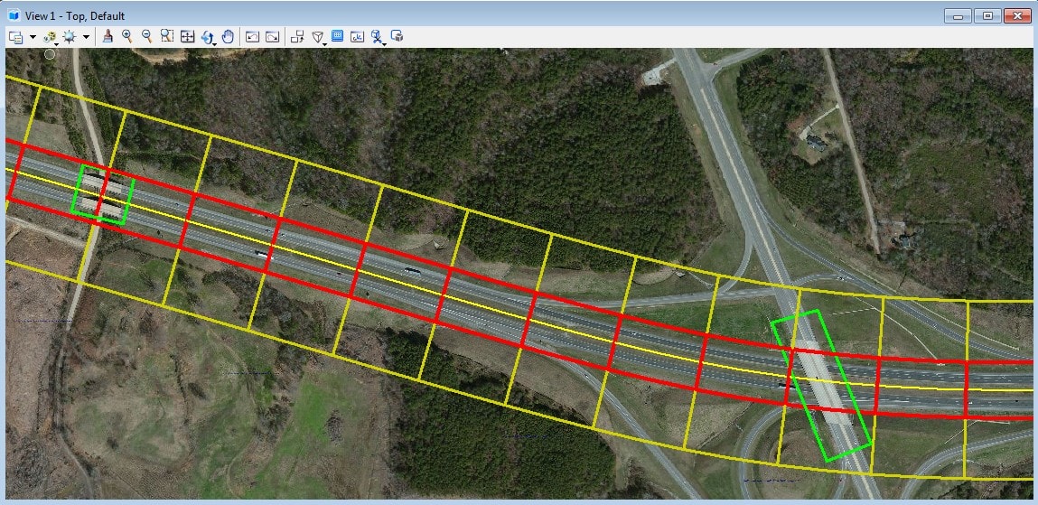
One can now use the comprehensive approach provided in this document to establish LiDAR requirements for each individual tile color. In the example above, LiDAR data requirements in the areas outside the highway edge might be optimally and cost-effectively acquired from an airborne LiDAR platform. Of course that same data would extend across the highway as well employing survey control along the highway surface for reference.
Along the highway, the fastest and most cost-effective means of acquiring the corridor data would probably be a terrestrial mobile LiDAR system. Note that mobile platforms typically require reference survey control coordinates every 500 to 1000 feet (152 to 205 meters) along the highway with extra control in areas of limited GPS. Further cost savings could be achieved by using this control for both airborne and terrestrial mobile system. Finally static based LiDAR systems might be optimal for the highest level of LiDAR requirements required around bridge structures. These scans might also share the same survey reference control as the airborne and terrestrial mobile LiDAR systems.
Below is a table summarizing the LiDAR data requirements across the entire project area. Data acquired from different LiDAR platforms is identified by color with requirements summarized by just a few parameters values. The resulting summary is elegantly simple yet very comprehensive.
Coverage RFP Requirement
The project overview is represented in the accompanying CAD illustration – see above. The area is subdivided by enclosed colored polygons. Data acquired within each polygon will meet the unique requirements assigned to the corresponding color. These requirements are summarized in the following table. Should colored areas overlap, the most stringent requirements assigned to an overlapping color will apply.
| Value | Comment | |
| Green | Static LiDAR Data | |
| Scan Alignment | Es = 0.03 ft (9 mm) P = 4% of total scans R = 80 ft |
Scan Alignment RFP Requirement (static) |
| Survey Control Alignment | Ec = 0.02 ft (6mm) (N/Es = 0.03 ft (9mm)) P = 4% of total scans r = 0.5 ft (30mm) |
Survey Control Alignment RFP Requirement (static topography) |
| Calibrated Image Alignment | Px = 2 pixels WxH = 12.1 megapixels FOV = 100 degrees |
Calibrated Image RFP Requirement |
| Random Noise | N = 0.04 ft (12mm) | Random Noise RFP Requirement |
| Point Density | D = 20 points / sq ft | Point Cloud Density RFP Requirement |
| Red | Mobile LiDAR Data | |
| Flightline Alignment | Ef = 0.05 ft (15 mm) M = 3 miles |
Flightline Alignment RFP Requirement (Mobile) |
| Survey Control Alignment | Elm = 0.05 ft (15mm) (N/Em = 0.1 ft (30mm)) P = 20% of corridor r = 0.05 ft (15mm) |
Survey Control Alignment RFP Requirement (Mobile) |
| Calibrated Image Alignment | Px = 5 pixels WxH = 2452 x 2056 pixels FOV = 80 x 65 degrees |
Calibrated Image RFP Requirement |
| Random Noise | N = 0.04 ft (12mm) | Random Noise RFP Requirement |
| Point Density | D = 20 points / sq ft | Point Cloud Density RFP Requirement |
| Yellow | Airborne LiDAR Data | |
| Flightline Alignment | Ef = 0.1 ft (30 mm) M = 3 miles |
Flightline Alignment RFP Requirement (Mobile) |
| Survey Control Alignment | Elm = 0.15 ft (45mm) (N/Em = 0.3 ft (90mm)) P = 20% of corridor R = 1.5 ft |
Survey Control Alignment RFP Requirement (Mobile) |
| Calibrated Image Alignment | Px = 2 pixels WxH = 7500 x 11500 pixels FOV = 40 x 30 degrees |
Calibrated Image RFP Requirement |
| Random Noise | N = 0.1 ft (30mm) | Random Noise RFP Requirement |
| Point Density | D = 5 points / sq ft | Point Cloud Density RFP Requirement |
Note: These values are typical and serve here as examples. Customers might survey Consultants for suggested values based on the application requirements. As always, the right balance between encouraging competitive bidding while avoiding data not meeting project requirements is the objective.
In this example, the optimal platform based on performance and cost was applied to each area in order to achieve the corresponding topography and model requirements. This information can now be easily communicated to one or more Consultants.
It should be noted that the aforementioned example was not an actual project. It was developed to represent the fundamental approach to developing the Coverage requirements. Every project will be unique in some way requiring the project team to maintain the appropriate levels of practicality and flexibility in defining Coverage requirements.
Summary
This document had been designed as a tutorial for the Customer seeking to develop requirements necessary for the successful acquisition of LiDAR data in support of an infrastructure project. The concepts, methods and techniques presented herein are not overly rigorous, yet have consistently proven reliable in assuring the acquired LiDAR data is of sufficient quality to meet project requirements.
The brief presentation of LiDAR data uncertainty provided the reader with an understanding of the methods for defining requirements as well as extracting quantifiable metrics for comparison against those requirements. Whenever relevant, practical metric extraction examples were presented using tools and techniques provided by TopoDOT® processing software. Each presentation of a data requirement included suggested text for inclusion into an RFP.
In conclusion, this document provides a customer with a practical and well-defined process for developing LiDAR data requirements, extracting quantifiable metrics from the data and incorporating such requirements into an RFP. It should be stressed that each individual project will have unique requirements. Thus these concepts, methods and tools should be applied with some flexibility. In the final analysis, this document reduces a seemingly complex undertaking to a straightforward process for any Customer wanting to exploit the benefits of LiDAR technology applied to an infrastructure or similar project.
The best way to make the most of LiDAR data is to use an effective point cloud processing software. TopoDOT software automates the entire process — making working with LiDAR easier than ever. Sign up for a free demo today.
1 Comment
4 Types Of LiDAR Remote Sensing Explained - TopoDOT Blog · September 11, 2019 at 2:41 PM
[…] Mobile LiDAR systems are mounted to moving vehicles such as cars, trains, and boats. Rather than just using one laser, they can have several so they can scan multiple angles at the same time. […]